There are a bunch of simple tips and tricks as well as quick shortcuts, hacks, and time-saving workarounds in Microsoft Excel that can help you type less, save time and boost your productivity, no wonder if you are a beginner or an advanced user. Here are some of the useful and top 10 Microsoft Excel sheet tricks that you should know.

1) Enter 0 before any number
Sometimes it requires you to add 0 before some numbers in your Excel sheet, even though 0 before any number won’t make any sense, but in some cases, your sheet may look neater, more understandable, and gives you more clarity. So here is a very simple trick to add 0 before the number you enter in the cell.
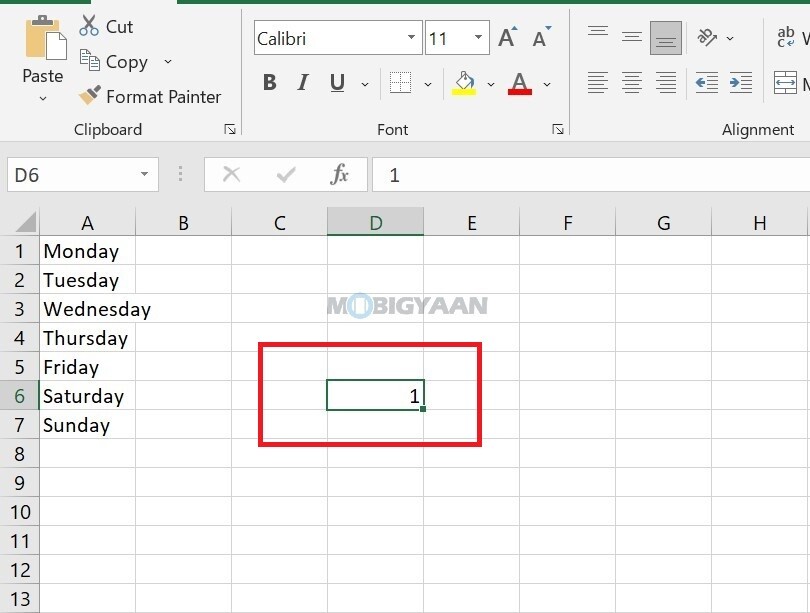
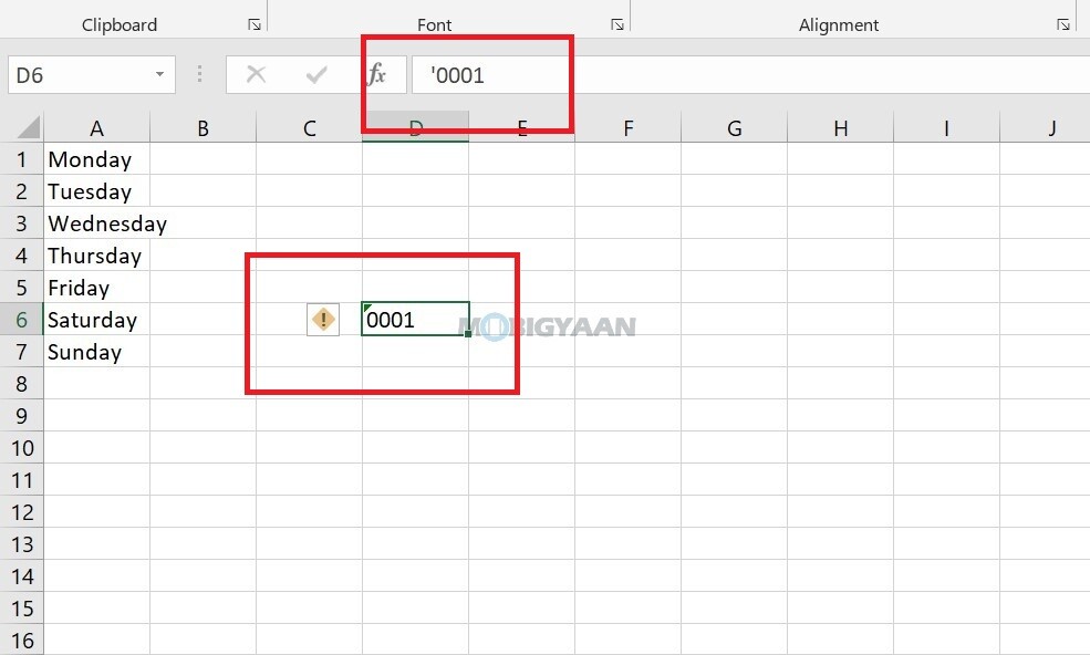
- To add a zero before any number, all you need to do is type in ‘ (single quote) before your zeros to enter them in a cell. For example, type ‘0001 to add this number 0001 in your sheet.
2) Transpose Your Cell Data
Sometimes you have big rows and fewer columns. It gives readers a complex view of your Excel Sheet. Here you can convert your rows into columns and columns to rows to have a sorted sheet. Take a look at this trick to transpose your sheet values.
- Step 1: Select the cells you want to Transpose.
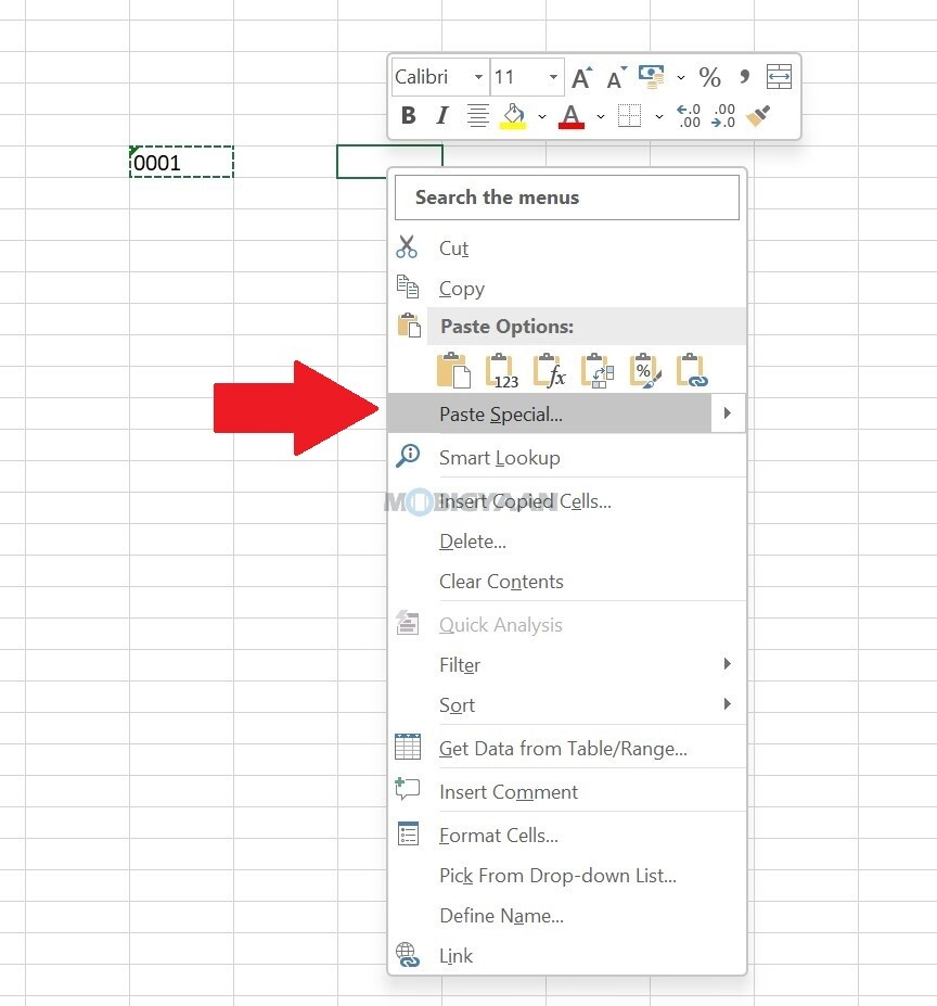
- Step 2: Right-click and copy the entire data.
- Step 3: Select the cell where you want your result to appear, right-click and choose Paste Special.
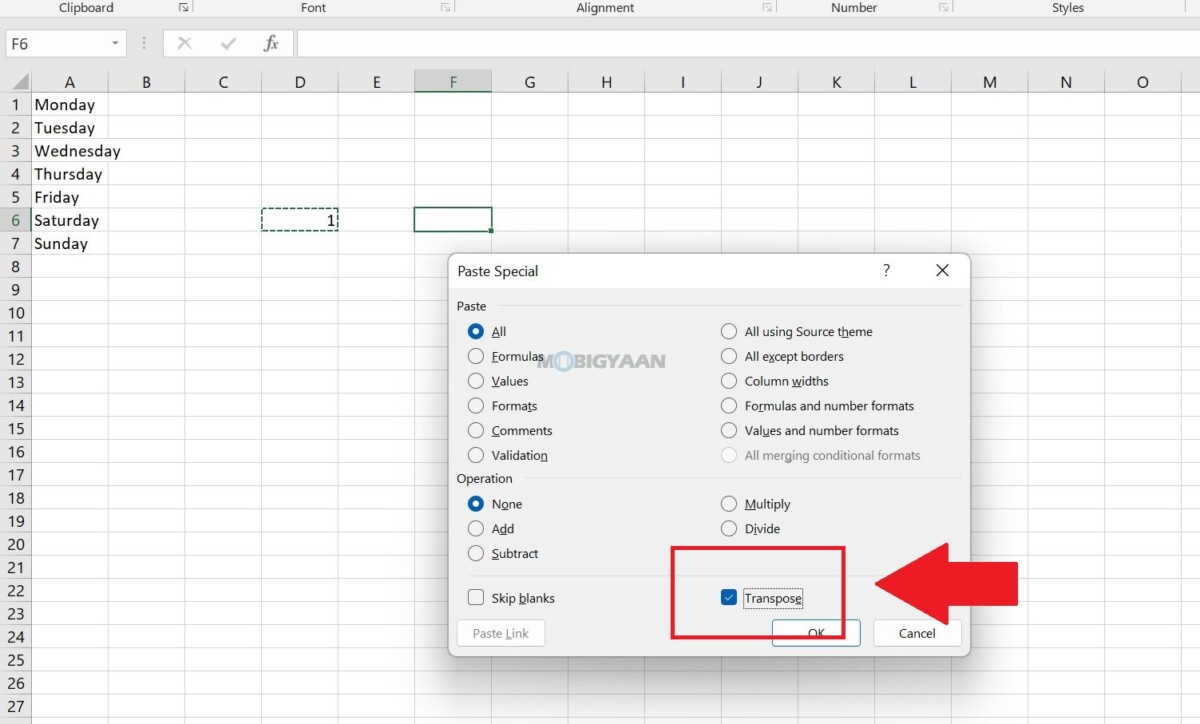
- Step 4: Now in the Paste Special window check the Transpose option.
3) Restrict data using Data Validation
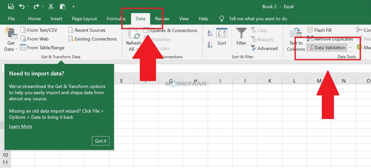
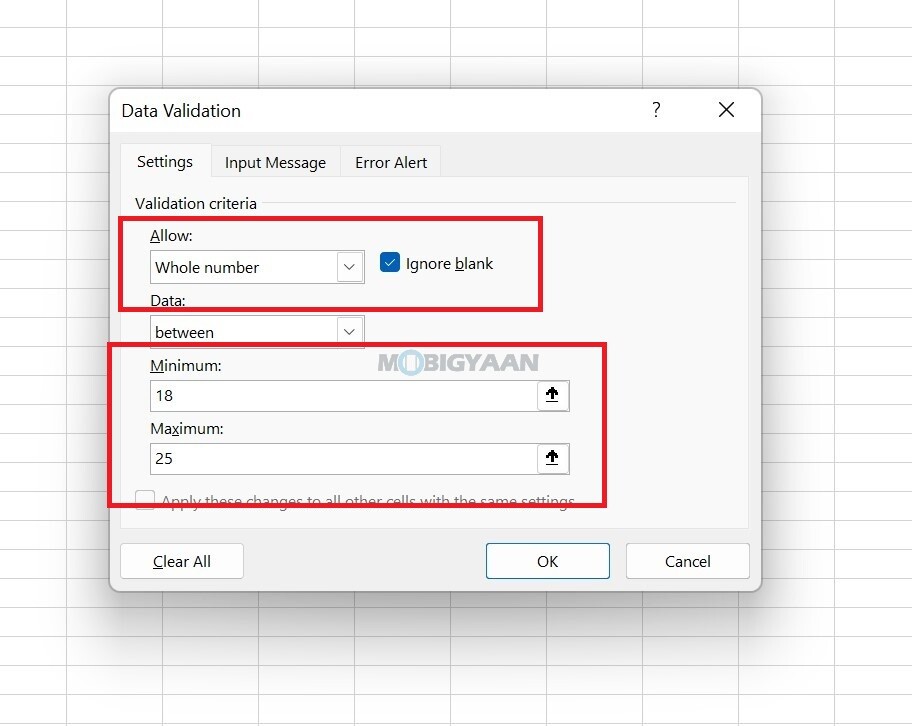
You can restrict the cell to input the data that only you have decided, such as a range or an age group. If you want to enter a specific age group like between 18 and 25, you can use the Data Validation function to restrict the cell from using any values beyond this range. Here’s how you can do it, follow these steps.
- Step 1: Select the Data tab and choose Validation.
- Step 2: In the validation window under the Settings section select Allow as the whole number and fill in other details as per your requirement.
- Step 3: Now go to Input message and type your error message here.
4) Create Your Own Shortcuts
If you are a speed user and want to quickly access the shortcuts, you can manually set your own. Generally, there are only three options available on the top toolbar – Save, Undo, and Redo. But you can create your own shortcuts like Copy, Paste, Print, and many more.
To set your own shortcut in Microsoft Excel, follow the steps below.
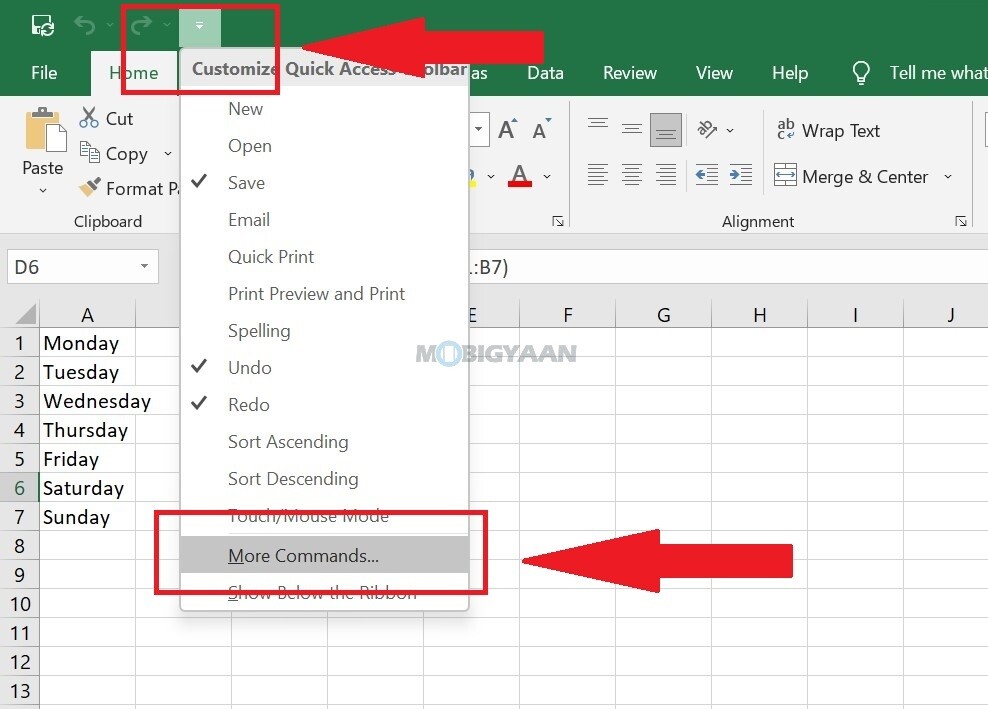
- Step 1: Launch the Micorosft Excel and in the top toolbar, click on the drop-down arrow as shown in the screenshot.
- Step 2: Click on More Commands from the menu and a window will open where you can set your own shortcuts.
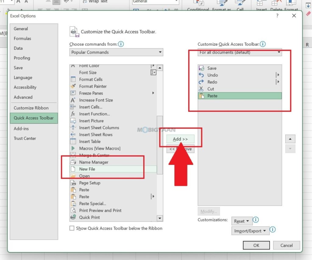
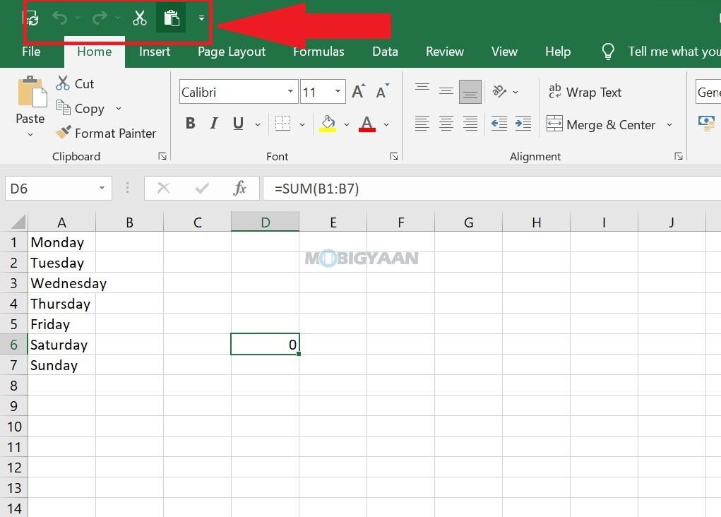
- Step 3: From here, you can choose the shortcuts that you want to keep in the toolbar, and click on Add to add your shortcuts. We have added Cut, and Paste as you can see in the image. You can access all these shortcuts from the top toolbar, clicking the arrow will give you more options.
5) Hide Your Formulas
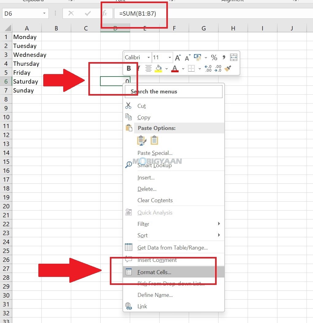
Want to hide your formulas in Microsoft Excel? The formulas that you have used are visible in the top preview bar and anyone can view them. When you hide the formulas, it also gives your Excel sheet a neater look. There’s a sneaky hack that you can use to hide your formulas in Microsoft Excel, just follow these simple steps.
- Step 1: Right-click on the cell that has a formula.
- Step 2: Choose the Format Cells option from the menu.
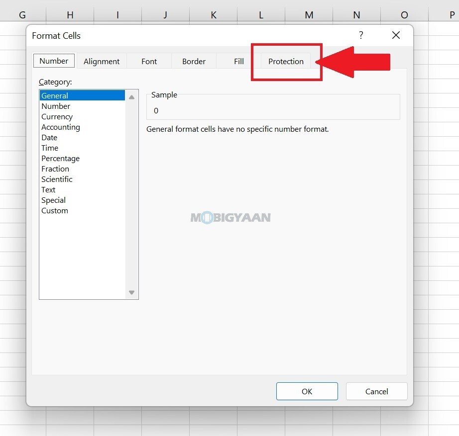
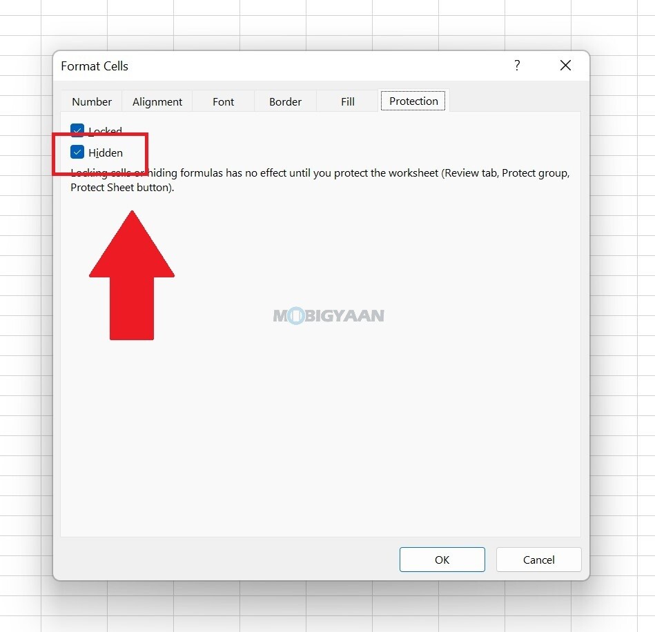
- Step 3: Under the Format Cells window, go to the Protection tab and check the box that says, Hidden.
- Step 4: Click on OK to save changes.
Once you have checked the Hidden box, it won’t hide right away if you haven’t protected the sheet. You need to protect the Excel sheet with a password in order to hide the formulas.
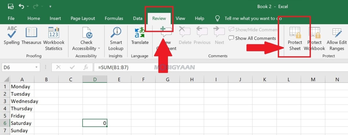
- Step 5: To protect the Excel sheet, head to the Review tab and click on Protect sheet.
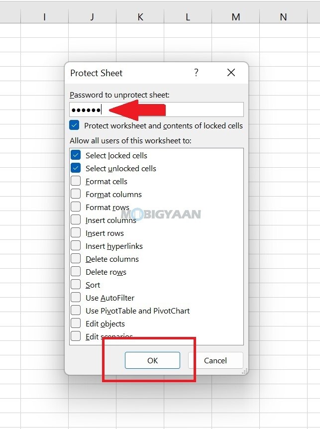
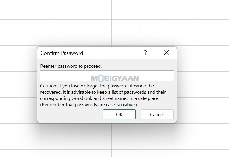
- Step 6: You will be asked to create a password for the sheet and then again you will be prompted to re-enter the password. Confirm it and click OK.
Make sure you remember the password otherwise you will lose the Excel sheet. You won’t be able to recover it if you forget the password. It is advisable to keep the password in a safe place.
6) Hide Cell Data
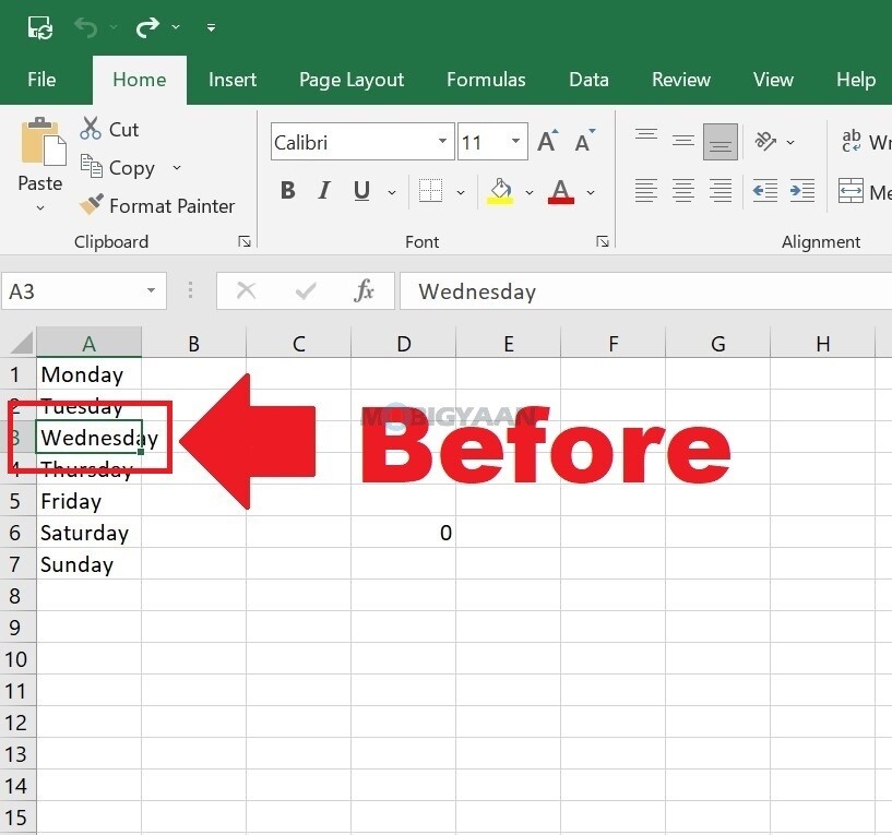
Similar to how you hide the formulas we have shown above, you can also hide the data entirely from the cell. Yes! And many of you don’t know about it. This nifty trick can be useful if you want to hide specific cell data or entire row/column data from the users who can access the Excel sheet. Here’s how you can do it.
- Step 1: Select the cell data you want to hide.
- Step 2: Right-click on it and choose Format Cells from the menu. You can also use CTRL + 1 to enter the Format Cells option.
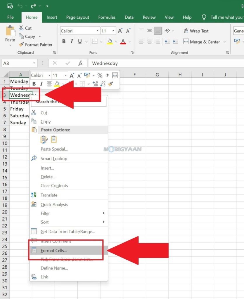
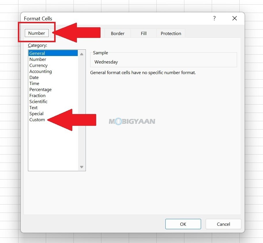
- Step 3: Under the Format Cells window, make sure you are in the Number tab. On the left side pane, go to the bottom and click on Custom.
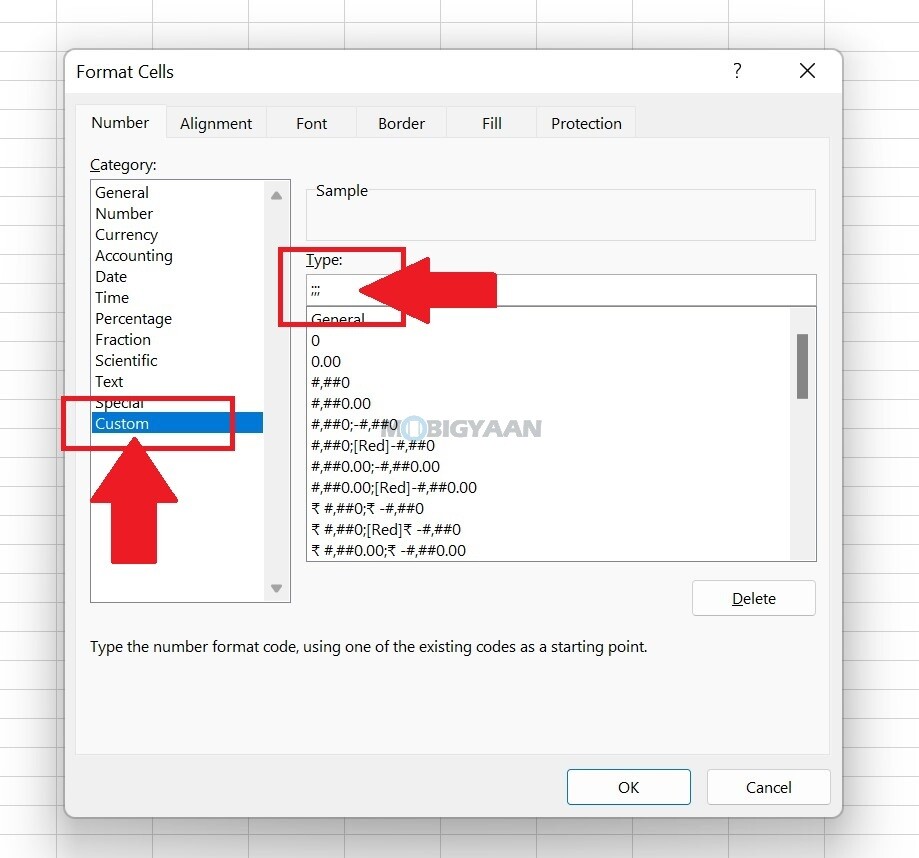
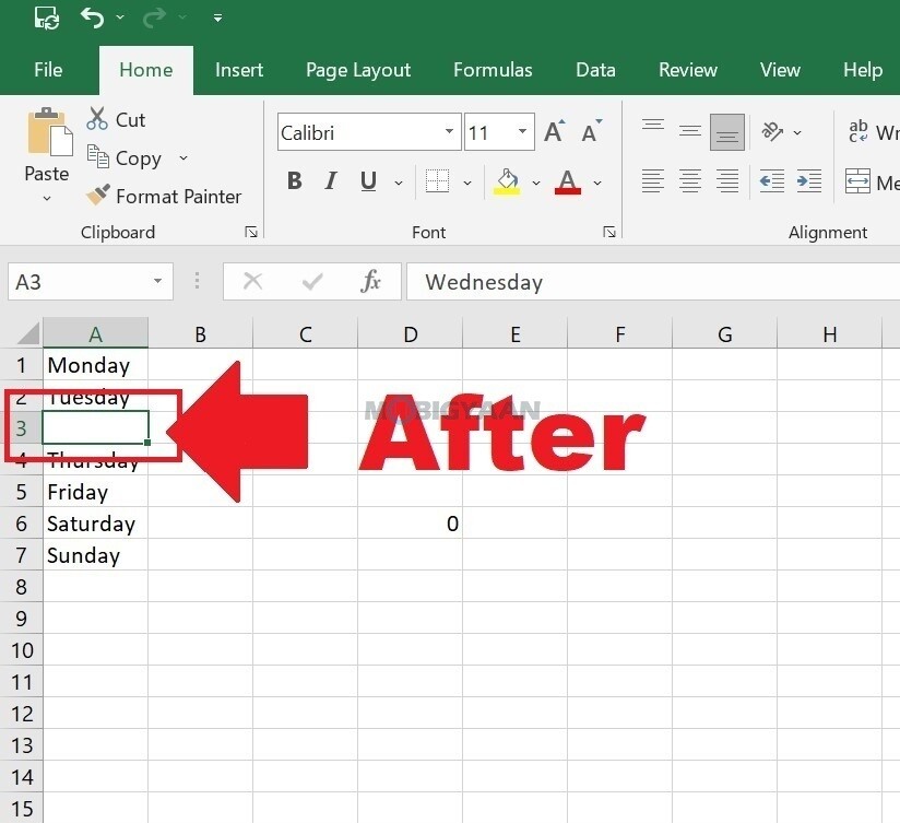
- Step 4: In Custom, type ;;; (three times) to hide the values from the cell. You can choose multiple cells and use the same trick to hide the data.
If you want to see the cell data, you can quickly view in the preview bar next to the function button in the top area. Although the cell data is visible in the preview bar and anyone can view it if they know, it’s still useful if people don’t notice the preview bar.
7) Insert A Drop-Down List
Adding a drop-down list in Microsoft Excel can save you time and type less, it also improves your productivity. If you are using repeated values in the cell, it’s better to choose from the drop-down menu rather than typing in every time. This makes things simple for you, saves you a number of rows, and also prevents you from filling up the wrong values. Take a look at how you can add a drop-down list in Excel.
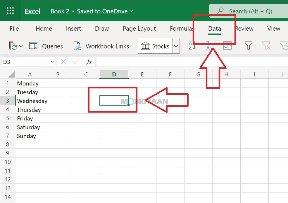
- Step 1: Select the Cell, the one that you want to make as a drop-down list.
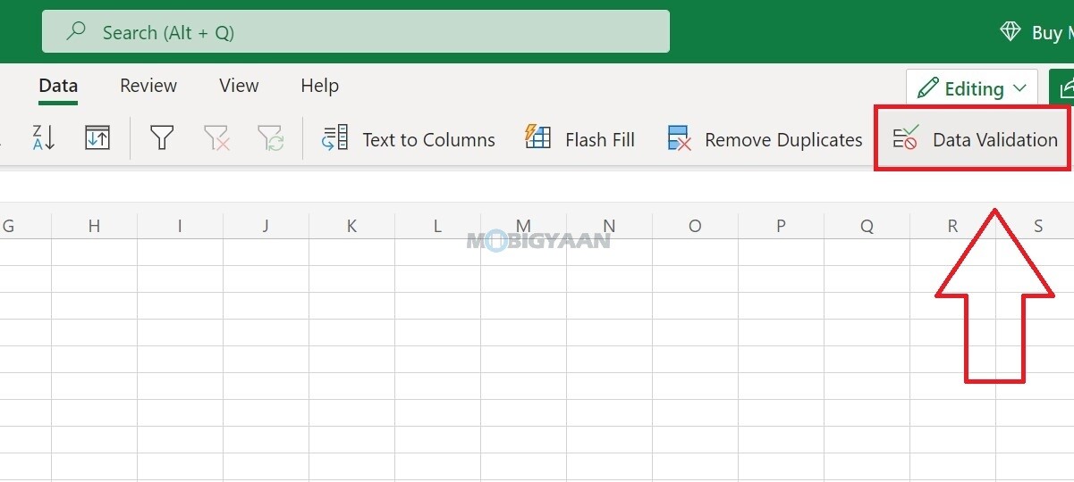
- Step 2: In the menu bar, click on Data and choose Validation.
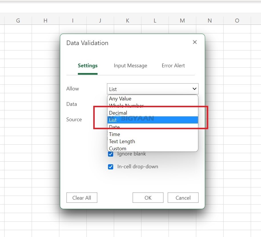
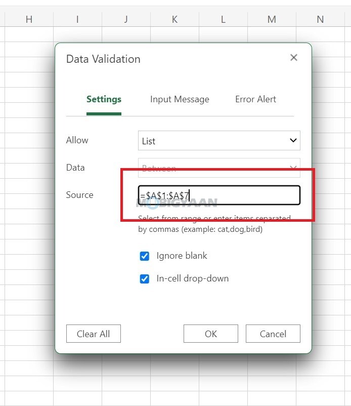
- Step 3: Under the Settings tab, you can see the Validation criteria. Here in the Allow field, choose List from the drop-down and type the cell source from where you are taking data to the list e.g. B1 to B10.
- Step 4: Click Ok to save and close the window.
Now the cell you have selected will be converted into a drop-down list that shows you the list of data you have sourced. Here’s the result, you can see the drop-down list in the image below.
Note: We have used Microsoft Excel using office.com, but the features remain very similar just as you use the dedicated Excel app.
That was it, these are some of the useful Microsoft Excel tips and tricks that can save you time. For more such content, visit our How-To Guides section. To get updates on the latest tech news, smartphones, and gadgets, make sure you follow us on our social media profiles.

